Robotics Nanodegree Project 4 - Deep Learning
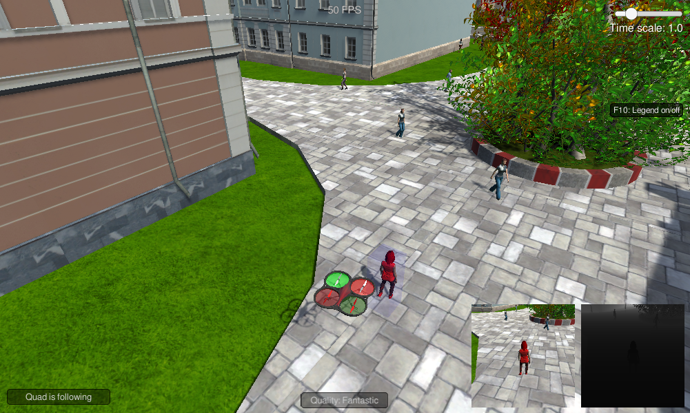
The deep learning project, also known as the Follow Me project, uses a fully convolutional network (FCN) to build a model for identifying a target person from a simulated drone camera feed. The purpose of the model is to have the drone follow the target person as they walk around, ignoring other non-target people.
The model is built within Tensorflow and Keras, and was trained using a K80 GPU enabled AWS compute instance.
To learn more about running the training code, view the original Udacity project repo here.
View the research Jupyter Notebook here.
Contents
Architecture
The project requires a model that is able to segment objects within the video stream. This means that each pixel in the image needs to be labeled. Fully convolutional networks (FCNs) are able to perform this in a process called semantic segmentation. Not only is the output the same size as the original input image, but each pixel in the output image is colored one of N segmentation colors.
By using semantic segmentation, FCNs are able to preserve spatial information throughout the network.
Fully Convolutional Networks
CNNs and FCNs both have an encoder section compromised of regular convolutions, however, instead of a final fully connected layer, FCNs have a 1x1 convolution layer and a decoder section made of reversed convolution layers. This means the FCNs are assembled with all layers being convolutional layers.
Encoder
The encoder section is comprised of one or more encoder blocks, each of which includes a separable convolution layer.
Separable convolution layers are a convolution technique for increasing model performance by reducing the number of parameters in each convolution. Put simply, this is achieved by performing a spatial convolution while keeping the channels separate, followed with a depthwise convolution. Instead of traversing the each input channel by each output channel and kernel, separable convolutions traverse the input channels with only the kernel, then traverse each of those feature maps with a 1x1 convolution for each output layer, before adding the two together. This technique allows for the efficient use of parameters.
Each encoder layer allows the model to gain a better understanding of the shapes in the image. For example, the first layer is able to discern very basic characteristics in the image, such as lines, hues and brightness. The next layer is able to identify shapes, such as squares, circles and curves. Each subsequent layer continues to build more insight into the image. However, although each layer is able to gain a better understanding of the image, more layers increase the computation time when training the model.
1x1 Convolution Layer
By using a 1x1 convolution layer, the network is able to retain spatial information from the encoder. When using a fully connected layer, the data is flattened, retaining only 2 dimensions of information. Flattening the data like this is useful for classification, however, the model needs to be able to classify each pixel in the image. 1x1 convolution layers allow the network to retain this location information.
An additional benefit of 1x1 convolutions is that they are an efficient approach for adding extra depth to the model.
The 1x1 convolution layer is simply a regular convolution, with a kernel and stride of 1.
Decoder
The decoder section of the model can either be composed of transposed convolution layers or bilinear upsampling layers.
The transposed convolution layers reverse the regular convolution layers, multiplying each pixel of the input with the kernel.
Bilinear upsampling uses the weighted average of the four nearest known pixels from the given pixel, estimating the new pixel intensity value. Although bilinear upsampling loses some finer details when compared to transposed convolutions, it has much better performance, which is important for training large models quickly.
The decoder block calculates the separable convolution layer of the concatenated bilinear upsample of the smaller input layer with the larger input layer. This structure mimics the use of skip connections by having the larger decoder block input layer act as the skip connection.
Each decoder layer is able to reconstruct a little bit more spatial resolution from the layer before it. The final decoder layer will output a layer the same size as the original model input image, which will be used for guiding the quad.
Skip Connections
Skip connections allow the network to retain information from prior layers that were lost in subsequent convolution layers. Skip layers use the output of one layer as the input to another layer. By using information from multiple image sizes, the model is able to make more precise segmentation decisions.
Model Used
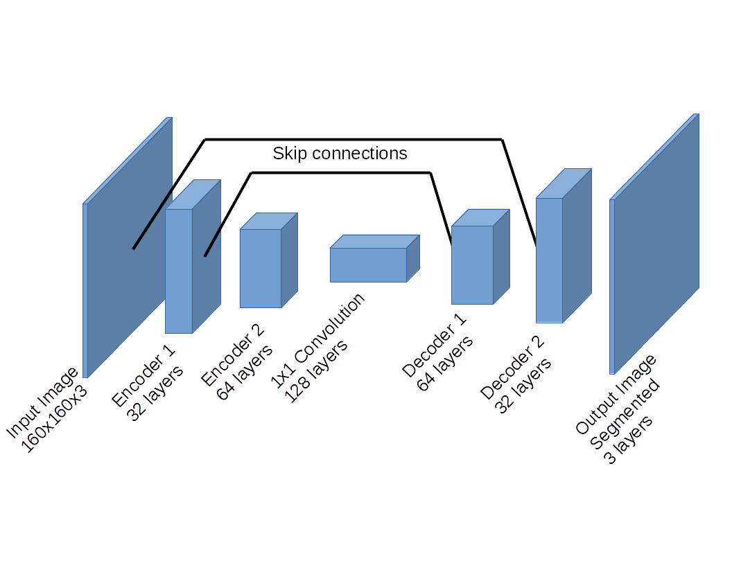
The actual FCN model consists of two encoder layers, the 1x1 convolution layer, and two decoder block layers.
The first convolution uses a filter size of 32 and a stride of 2, while the second convolution uses a filter size of 64 and a stride of 2. Both convolutions used same padding. This padding combined with a stride of 2 causes each layer to halve the image size, while increasing the depth to match the filter size used.
The 1x1 convolution layer uses a filter size of 128, with the standard kernel and stride size of 1.
The first decoder block layer uses the output from the 1x1 convolution as the small input layer, and the first convolution layer as the large input layer. A filter size of 64 is used for this layer.
The second decoder block layer uses the output from the first decoder block as the small input layer, and the original image as the large input layer. This layer uses a filter size of 32.
Finally, a convolution layer with softmax activation is applied to the output of the second decoder block.
I found that making the model deeper resulted in worse performance and longer training times. I did this by adding both an extra convolution layer and an extra decoder block layer, each with a filter size of 256. Therefore, I stuck with a model with 2 convolutions and 2 decoder layers.
Hyperparameters
The optimal hyperparameters I found (for the time taken) are:
- learning rate = 0.001
- batch size = 100
- number of epochs = 10
- steps per epoch = 200
- validation steps = 50
- workers = 2
I found that a batch size larger than 100 overflowed either the CPU or GPU cache, causing the system to write the extra information to RAM, slowing the training down. This makes sense because the larger epoch size requires more space.
The more epochs trained with always increased the model accuracy, however, there is a point of diminishing returns between accuracy and time required. I found that after 10 to 20 epochs, the accuracy only improved marginally. Every time the number of epochs is doubled, the training time is also doubled. Thus, I found that 10 epochs resulted in acceptable scores for the time taken.
Increasing the steps per epoch and validation only marginally increased the model accuracy, however, they drastically increased the training time. Thus it did not make sense to increase them beyond 200 and 50, respectively. Conversely, halving the values to 100 and 25, respectively, dramatically hurt the model's performance, while decreasing training time. Therefore, I stuck with 200 for the steps per epoch and 50 for the validation steps.
All of these hyperparameters were evaluated by manual tuning. In the future, I will implement either a grid search or a random search to aid this process.
Training
I trained the model on AWS using a p2.xlarge instance (Nvidia K80 GPU with 4 vCPUs and 61 GB of RAM). Training the model with the above hyperparameters required about 226 seconds per epoch, or about 38 minutes for the 10 epochs I used.
Performance
The final score of my model is 0.441, while the final IoU is 0.575.
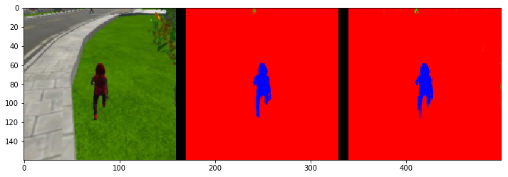
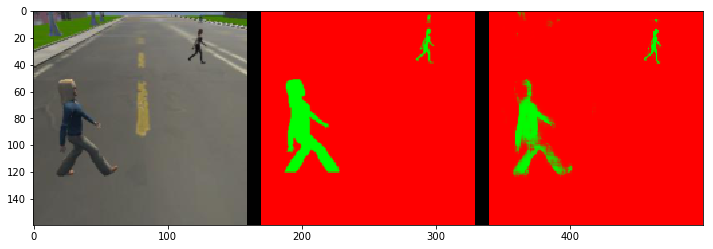
Here are some test images of the model output. The left frame is the raw image, the middle frame is goal, and the right frame is the output from the model. The objective is to have the right frame as close as possible to the middle frame. If the target person is identified, they are shaded in blue. The non-target people are shaded in lime green.
When following the target at close range, the model had an IoU for the target of 0.895, which is pretty good. The frames below show the model's output:
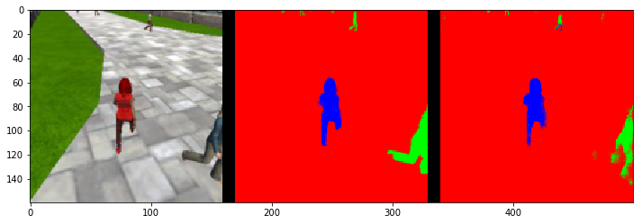
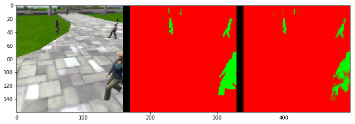
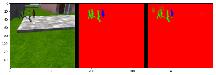
When the target person was not in the frame, the model had an IoU for identifying other people of 0.709. Here are some test images showing these results:
Finally, when the target was at a long distance, the model had an IoU for the target of 0.255, which isn't that good. This is a challenging test. These frames show the model's outputs for these images:
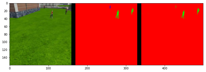
As you can see from the long range images, the model has difficultly at long distances. Additional training images might improve it's accuracy.
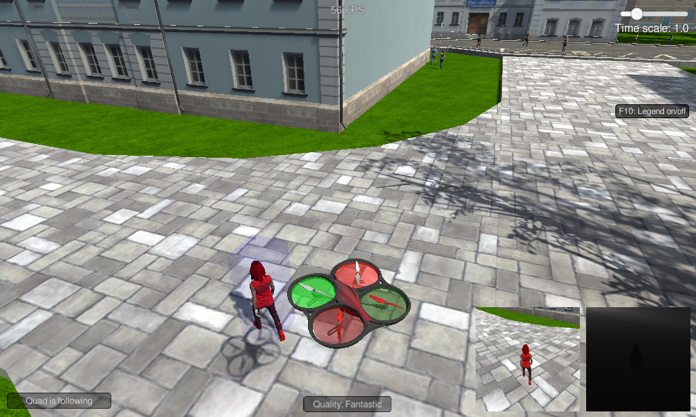
Ultimately though, the model was good enough that the quad had no trouble finding and following the target person in the simulated environment.
Future Enhancements
This model was exclusively trained on people, however, it could be altered for other object detection. For example, it could be trained on images of cars or animals. It is important to note that this would require the model to be trained from scratch. The model I trained in this project would not have good performance if it were simply given images of different objects to evaluate.
Training the model on new objects would require a large collection of training and validation images of the new object.
Research Notebook
To view the instructions for running the model, read this.
You can access the Jupyter Notebook I used to train the model here.