Robotics Nanodegree Project 3 - 3D Perception
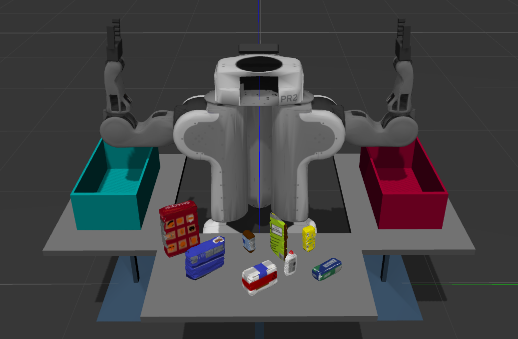
The third project of the Udacity Robotics Nanodegree focused on 3D perception using a PR2 robot simulation in Gazebo. The robot used a RGB-D camera to capture the color and depth of objects within its field of view. A SVM was used to train a model that was used to recognize what each object was. With each object identified, the robot was able to pick and place each object into the correct bin based on prior instructions.
The goal of perception is to convert sensor input into a point cloud image that can be used to identify specific objects, allowing the system to make decisions as to what should happen with each object. The three main parts of perception include filtering the point cloud, clustering relevant objects, and recognizing objects.
Filtering
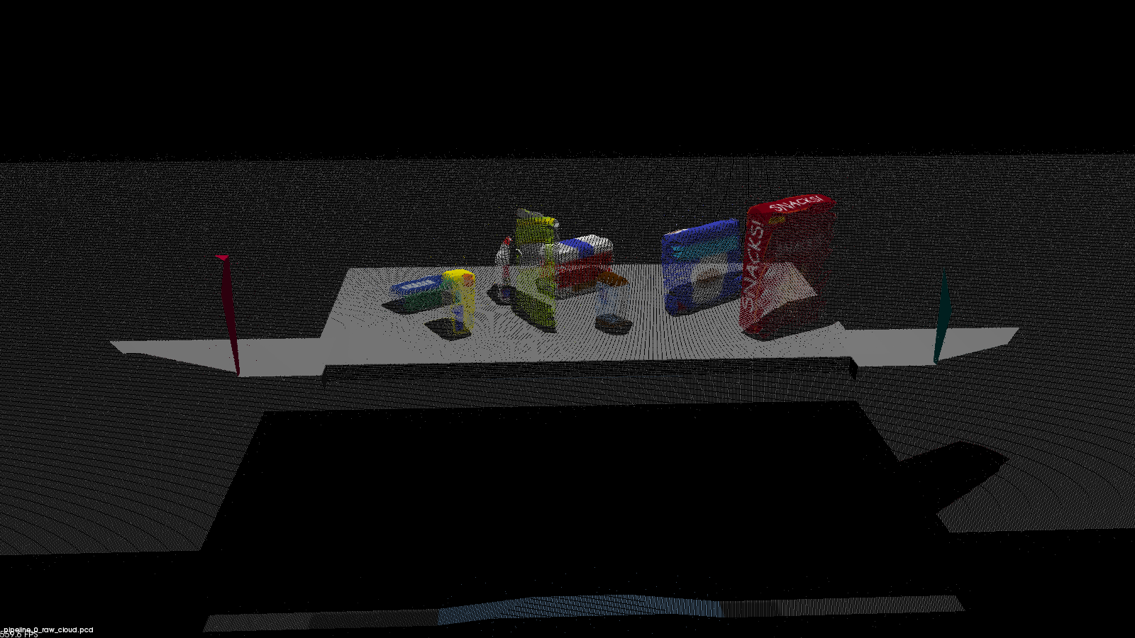
The first part of the perception pipeline filters the raw point cloud to keep only the essential data, removing adversarial data points and compressing the cloud data.
The raw point cloud object from the PR2 simulation looks like this:
Outlier Removal Filter
Outlier filters can remove outliers from the point cloud. These outliers are often caused by external factors like dust in the environment, humidity in the air, or presence of various light sources. One such filter is PCL's StatisticalOutlierRemoval filter that computes the distance to each point's neighbors, then calculates a mean distance. Any points whose mean distances are outside a defined interval are removed.
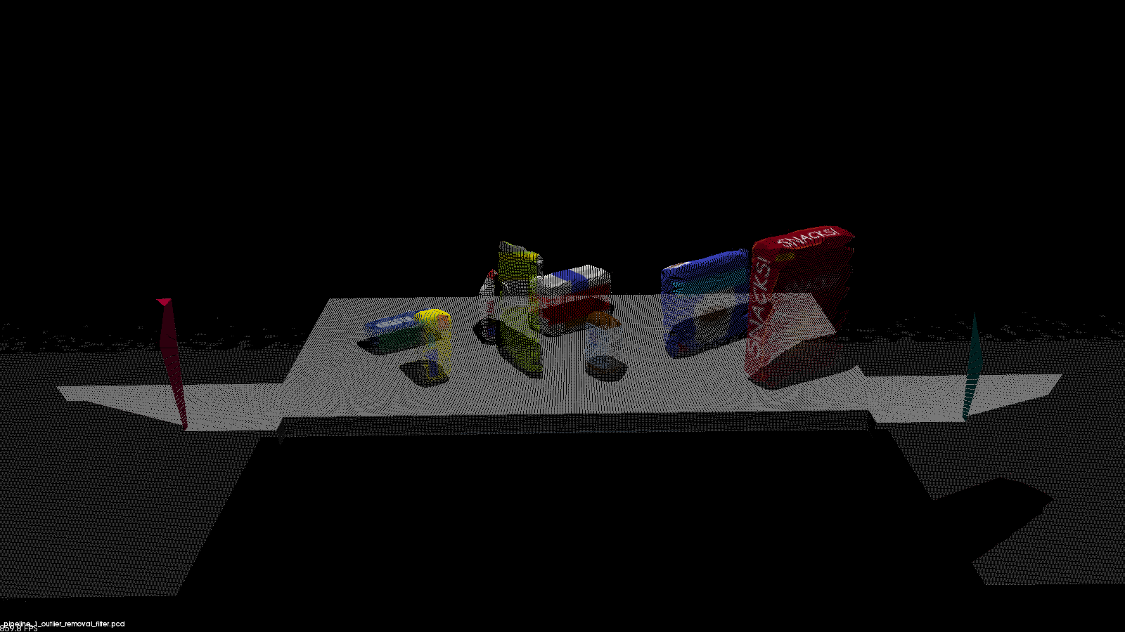
For the PR2 simulation, I found that a mean k value of 20, and a standard deviation threshold of 0.1 provided the optimal outlier filtering.
Here is the cloud after performing the outlier removal filter.
Voxel Grid Filter
The raw point cloud will often have more details than required, causing excess processing time when analyzing it. A voxel grid filter down-samples the data by taking a spatial average of the points in the cloud confined by each voxel. The set of points which lie within the bounds of a voxel are assigned to that voxel, and are statistically combined into one output point.
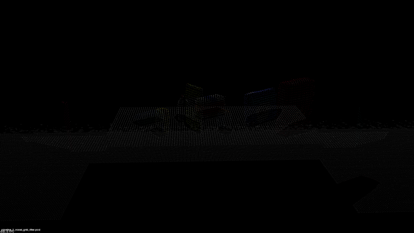
I used an X, Y, and Z voxel grid filter leaf size of 0.01. This value represents the voxels per cubic meter, thus increasing the number adds more detail and processing time. Using 0.01 was a good compromise of leaving enough detail while minimizing processing time, however, increasing the number would increase the model's accuracy (and increase processing time).
Here is the cloud after using the voxel grid filter:
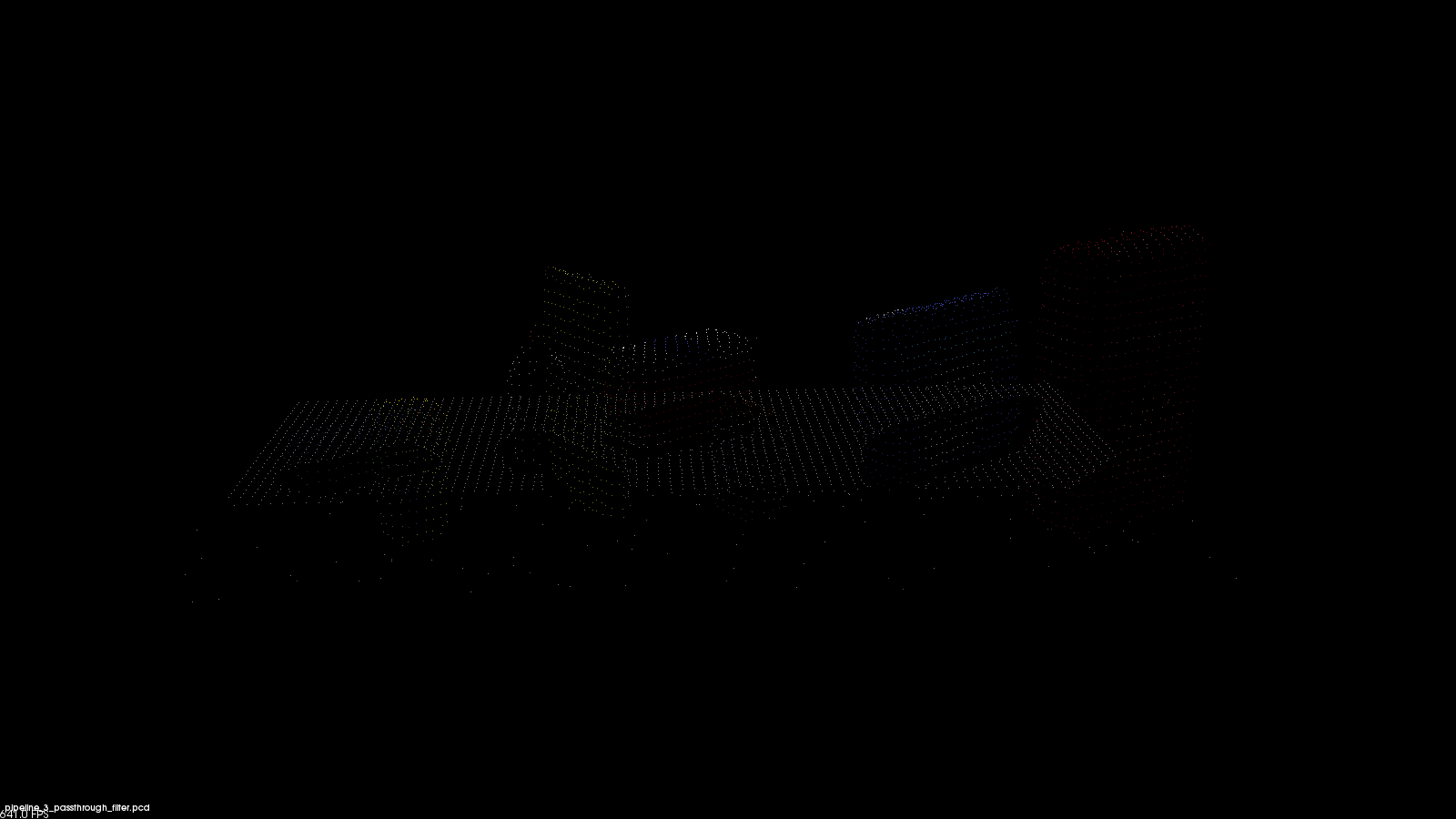
Passthrough Filter
The passthrough filter allows a 3D point cloud to be cropped by specifying an axis with cut-off values along the axis. The region allows to pass through is often called the region of interest.
The PR2 robot simulation required passthrough filters for both the Y and Z axis (global axis). This prevented processing values outside the area immediately in front of the robot. For the Y axis, I used a range of -0.4 to 0.4, and for the Z axis, I used a range of 0.61 to 0.9.
Here is the point cloud after using the passthrough filter:
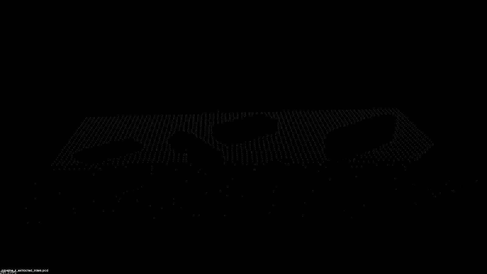
RANSAC Place Segmentation
Random Sample Consensus (RANSAC) is used to identify points in the dataset that belong to a particular model. It assumes that all of the data in a dataset is composed of both inliers and outliers, where inliers can be defined by a particular model with a specific set of parameters, and outliers don't.
I used a RANSAC max distance value of 0.01.
The extracted inliers included the table. It looks like this:
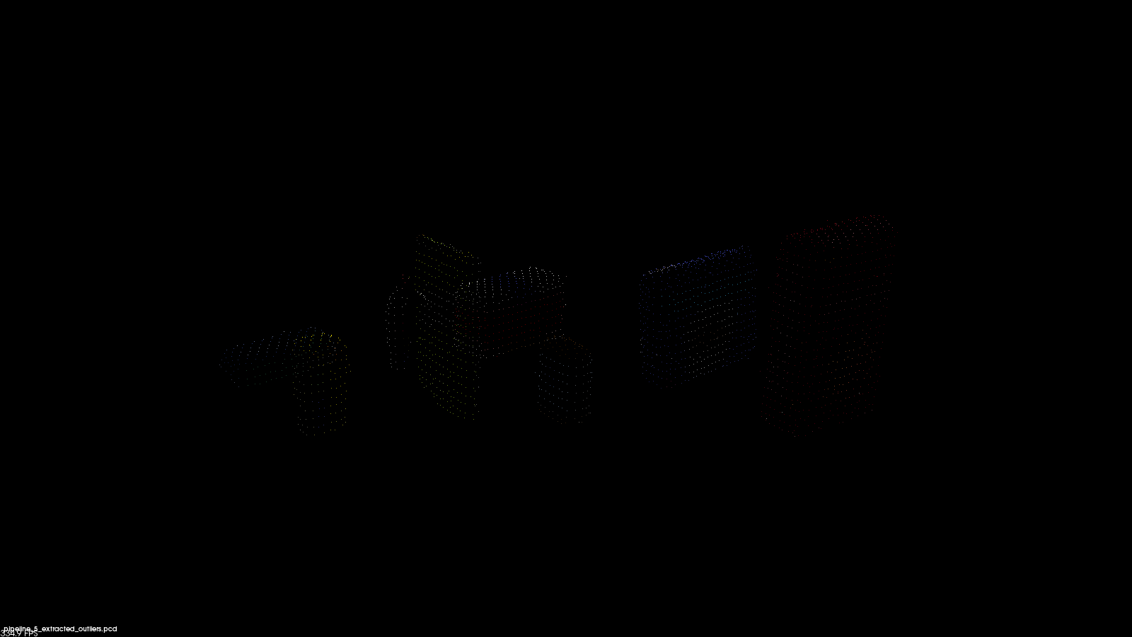
The extracted outliers contained the objects on the table. It looks like this:
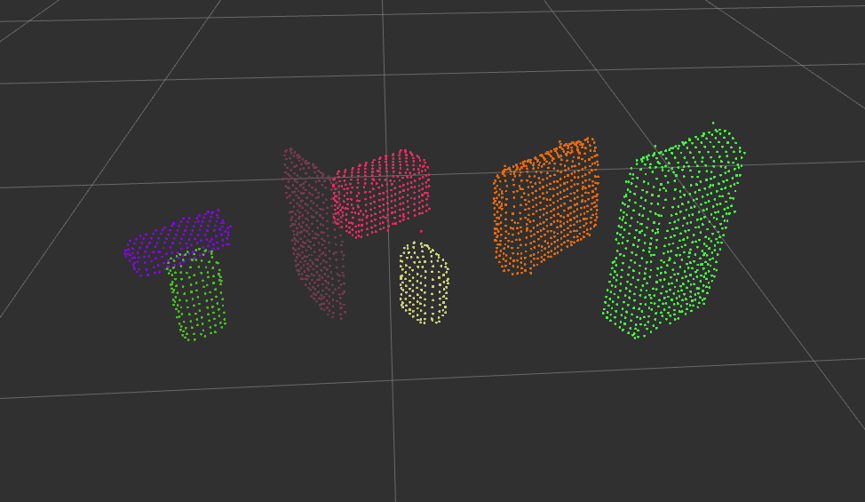
Clustering for Segmentation
With a cleaned point cloud, it is possible to identify individual objects within it. One straightforward approach is to use Euclidean clustering to perform this calculation.
The two main algorithms possible include:
- K-means
- DBSCAN
K-means
K-means clustering algorithm is able to group data points into n groups based on their distance to randomly chosen centroids. However, K-means clustering requires that you know the number of groups to be clustered, which may not always be the case.
DBSCAN
Density-based spatial cluster of applications with noise (DBSCAN) (sometimes called *Euclidean clustering*) is a clustering algorithm that creates clusters by grouping data points that are within some threshold distance from their nearest neighbor.
DBSCAN is unique over k-means because you don't need to know how many clusters to expect in the data. However, you do need to know something about the density of the data points being clustered.
Performing a DBSCAN within the PR2 simulation required converting the XYZRGB point cloud to a XYZ point cloud, making a k-d tree (decreases the computation required), preparing the Euclidean clustering function, and extracting the clusters from the cloud. This process generates a list of points for each detected object.
By assigning random colors to the isolated objects within the scene, I was able to generate this cloud of objects:
Object Recognition
The object recognition code allows each object within the object cluster to be identified. In order to do this, the system first needs to train a model to learn what each object looks like. Once it has this model, the system will be able to make predictions as to which object it sees.
Capture Object Features
Color histograms are used to measure how each object looks when captured as an image. Each object is positioned in random orientations to give the model a more complete understanding. For better feature extraction, the RGB image can be converted to HSV before being analyzed as a histogram. The number of bins used for the histogram changes how detailed each object is mapped, however too many bins will over-fit the object.
The code for building the histograms can be found in features.py.
The capture_features_pr2.py script saved the object features to a file named training_set_pr2.sav. It captured each object in 50 random orientations, using the HSV color space and 128 bins when creating the image histograms.
Train SVM Model
A support vector machine (SVM) is used to train the model (specifically a SVC). The SVM loads the training set generated from the capture_features_pr2.py script, and prepares the raw data for classification. I found that a linear kernel using a C value of 0.1 builds a model with good accuracy.
I experimented with cross validation of the model and found that a 50 fold cross validation worked best. A leave one out cross validation strategy provided marginally better accuracy results, however, it required much longer to process.
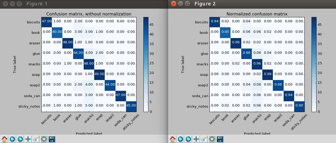
In the end, I was able to generate an accuracy score of 92.17%. The train_svm.py script trained the SVM, saving the final model as model.sav.
The confusion matrices below shows the non-normalized and normalized results for a test case using the trained model generated above.
PR2 Robot Simulation
The PR2 robot simulation has three test scenarios to evaluate the object recognition performance. The following sections demonstrate each scenario.
Test 1
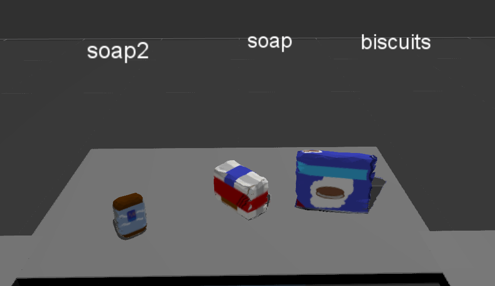
View the goal pick list, and the calculated output values.
Test 2
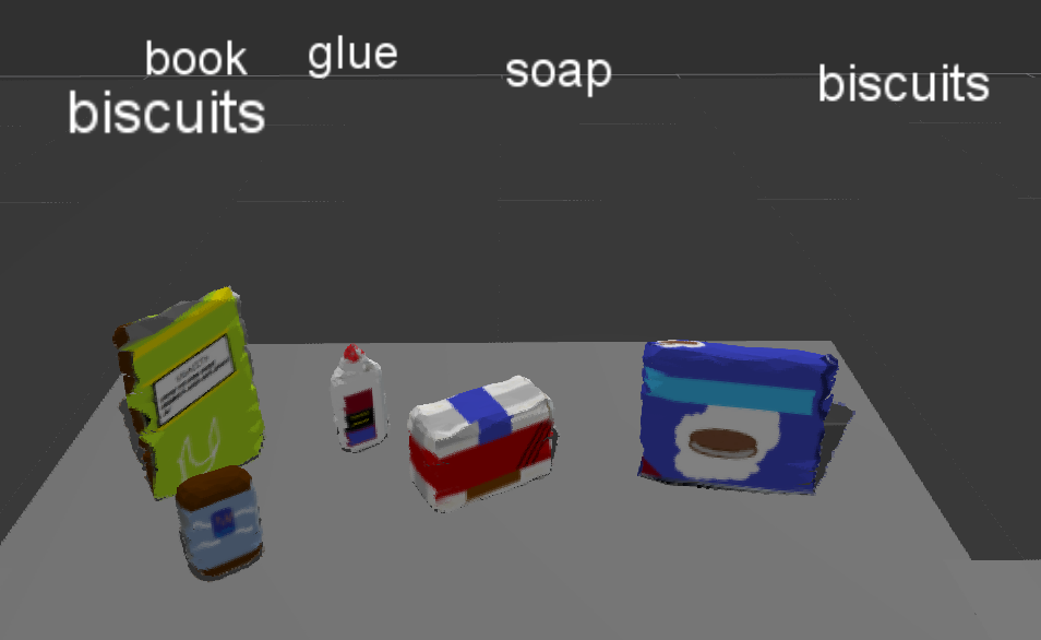
View the goal pick list, and the calculated output values.
Test 3

View the goal pick list, and the calculated output values.
Future Work
This project can be expanded to get the PR2 to actually grab each object and drop it to the correct bin. I have most of the code required to get this working, however, I need to finish the code that adjusts the collision map to remove each object that is to be picked up. Otherwise, the robot will never pick up the objects because it thinks it will collide with them.
Code Sources
The original Udacity perception exercise code can be found here. To install the exercise data on your own computer, view the installation guide here.
The PR2 3D perception project code source can be found here. Follow the instructions in the README.md to get the demo code working.
Run the Simulation
View the instructions here to get the code mentioned above working.