Robotics Nanodegree Project 2 - Pick and Place
The second project of the Udacity Robotics Nanodegree was the most challenging project I've done with Udacity over the past 3 years covering dozens of their courses. The project required writing the code to direct a simulated Kuka KR210 6 DoF arm to pickup a can from a shelf and place it within a bin next to the robot. A simple sounding task that required lots of work.
In addition to kinematics being new to me, I found the course guidance very lacking. They covered the basic theory of what needed to be done, but not enough details on the technical implementation. This meant I had to do a lot of self learning. That's nothing too unusual for me, but it just requires extra time. In total, I've been working on this project for the past 5 weeks!
For the project, the locations of the can and the bin were already known, thus inverse kinematics is used to calculate what angles each joint of the robot should be in to put the arm's gripper in the right position and orientation to grab and release the can. I used the Denavit-Hartenberg convention to aid this process.
Denavit-Hartenberg
The modified Denavit-Hartenberg (DH) convention aids in performing kinematic analysis for robotic systems. DH parameters allow four parameters to indicate the location and orientation of subsequent arm links instead of the 12 parameters required through the use of a homogeneous transformation matrix.
This table includes all of the DH parameters for the arm that were sourced from the arm's specifications.
| n | θ | d | a | α |
|---|---|---|---|---|
| 0 | - | - | 0 | 0 |
| 1 | θ1 | 0.75 | 0.35 | -90 |
| 2 | θ2 | 0 | 1.25 | 0 |
| 3 | θ3 | 0 | -0.054 | -90 |
| 4 | θ4 | 1.5 | 0 | 90 |
| 5 | θ5 | 0 | 0 | -90 |
| 6 | θ6 | 0.303 | 0 | 0 |
With these parameters, I was able to build this diagram of all arm joints and links.

With this diagram, it is possible to work on the kinematics of the arm.
Kinematics
Kinematics is the study of movement in a system, and not about the forces involved with that movement. Kinematics is heavily used within robotics for the purpose of measuring robotic arm movements. There are two areas of kinematics: forward kinematics and inverse kinematics.
Forward Kinematics
Forward kinematics uses the joint angles to derive the position and orientation of the end effector (gripper) of the robot after it moves. This process is relatively easy to calculate, requiring linear algebra to calculate and manipulate homogeneous transformation matrices, which are a combination of rotation matrices and displacement vectors.
Rotation matrices are 3 x 3 matrices that represent the 3D orientation of an object. These orientations are often referred to as roll, pitch and yaw.
The displacement vectors are a 3 x 1 vector that represent the 3D position of an object. These values are the X, Y, and Z values of an object.
The combination of the rotation matrix and displacement vector creates a homogeneous transformation matrix. This matrix is a 4 x 4 matrix, with the rotation matrix making up the top left 3 x 3 cells, and the displacement vector making up the top right 3 x 1 cells. The bottom row of the matrix contains [0, 0, 0, 1], which is used as a filler, so the matrix can be 4 x 4 in size for easier computation.
Each joint has its own homogeneous transformation matrix. Multiple homogeneous transformation matrices can be multiplied together to determine the position and orientation from the first matrix's object to the final matrix's object (i.e. from the base to the end effector). This is forward kinematics.
Inverse Kinematics
Inverse kinematics is much more involved than forward kinematics. With inverse kinematics, the end effector's position and orientation is already known, but the joint angles need to be found. This is a non-linear problem, thus it can't be solved analytically (i.e. by using the forward kinematics matrices in reverse). The two main approaches for solving inverse kinematics is to use a numerical approach, or a geometric approach (graphical method). I used the geometric approach below.
The geometrical approach uses trigonometric calculations to derive the appropriate angles needed for each joint. These calculations can be found by drawing the 3D arm in a 2D frame where normal trigonometric rules apply.
The following image shows the trigonometric diagrams I used to derive the right calculations to get the first three joint angles.

This diagram only has calculations for the first three joints, which determine the end effector's position. The last three joints are used to get the orientation of the end effector. These last three joints are commonly referred to as a spherical wrist since they can orient the end effector in any direction required.
I calculated the inverse kinematic orientation by first calculating the rotation matrix for joints 4, 5 and 6. Once I had this rotation matrix, I was able to calculate the Euler angles that represent the joint angles required.
I used a tf transformations function called euler_from_matrix that takes a numpy rotation matrix and Euler axis definition, and returns the three Euler angles (alpha, beta and gamma). The rotation matrix I provided used the Euler definition of XYZ, which is a Tait-Bryan angle combination. With the alpha, beta and gamma angles, I mapped them to θ4, θ5 and θ6, respectively. However, θ4 needed to have pi/2 added to it, and θ5 needed to be subtracted from pi/2.
Code
You can view the code I built for this project in this repository.
kuka_fk.py contains test code covering forward kinematics. This code can build transformation matrices for each arm joint.
kuka_ik.py contains test code covering the inverse kinematics of the project. It uses the predetermined trigonometric calculations to determine the correct joint angles the arm should use to place the end effector in the right position.
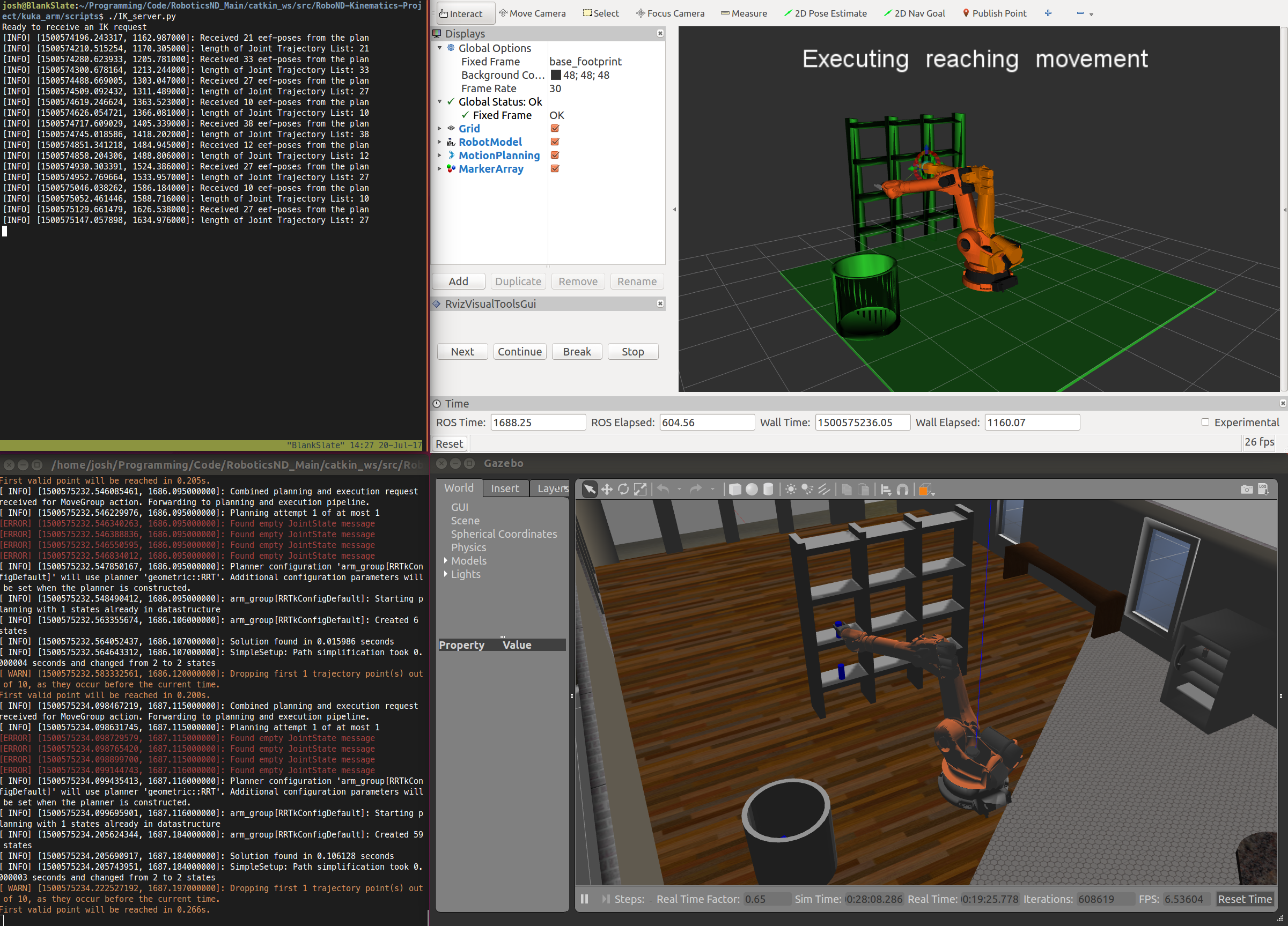
IK_server.py contains code that links into the ROS/Gazebo/Rviz simulator. To run the simulator, you first need to install this Udacity Kinematics Project code. View the notes here for more details on getting the IK_server.py code running with the simulator.
Next Step
Now that I've learned the basics of using kinematics to control a robotic arm, the next step is to use that knowledge to work with an actual arm. I've already ordered a simple 6 axis arm that uses hobby servos and an Arduino to run. That will be a fun challenge, so stay tuned for that!